CASI, SASI data processing

The data processing procedure is well apparent in the following charts showing the spectral characteristics of two sample pixels (vegetation, soil) in individual steps of the processing. Examples are given only for the VNIR spectral region.

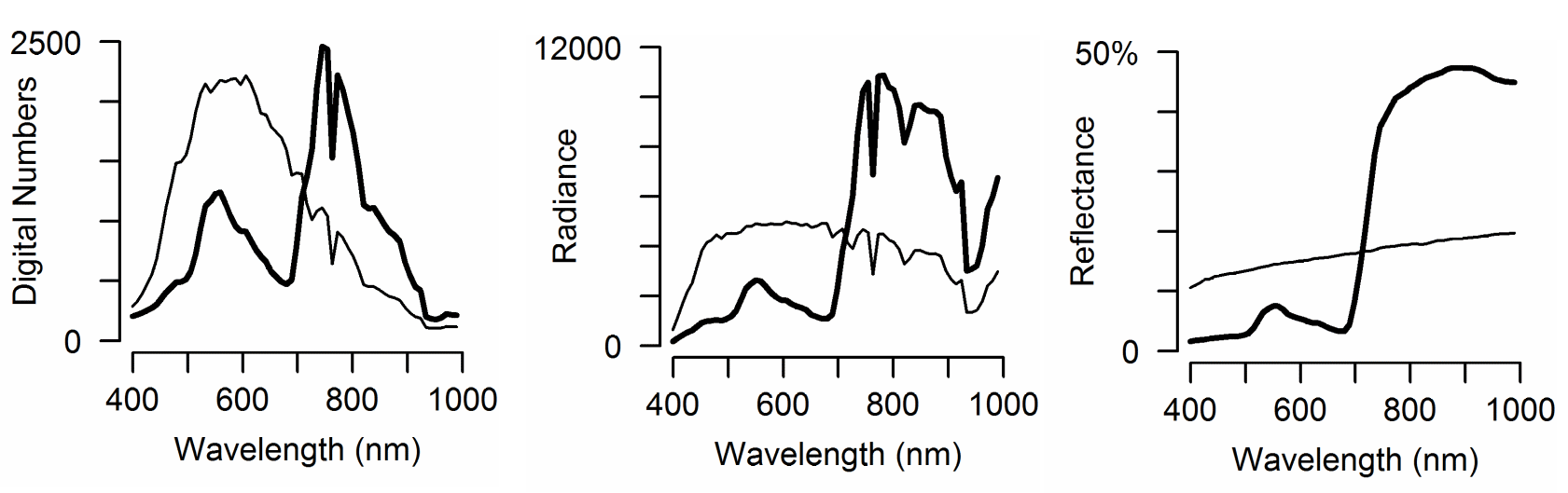
The spectral characteristics of two sample pixels (vegetation – bolder curve, soil – thinner curve) displayed in individual steps of the processing. The first chart shows the raw values (digital numbers) captured by the sensor. The second chart shows values converted to a physical quantity (radiance) after radiometric corrections. The third chart shows values after atmospheric corrections (reflectance).

Radiometric Corrections
The basic radiometric correction procedure consists in subtracting dark current and converting raw values scanned by the sensor (DN – digital numbers) into physically defined units of radiance. Radiometric corrections of measured data are carried out in RadCorr (Itres Ltd) using laboratory-determined calibration parameters that are determined for each pixel of the sensor matrix. The values of the final image data are given in radiometric units [μW cm-2 sr-1 nm-1] multiplied by 1000.

During radiometric corrections, it is possible to perform additional data corrections for effects that negatively affect the scanned hyperspectral data e.g.

Scattered light correction: Correcting the light scattered in the optical sensor system is especially important for the CASI-1500 sensor. Correction is carried out for individual rows. The amount of scattered light is detected using defined chip columns that are not reached by the image signal.

Frame Shift Smear Correction: Correcting the added signal that arises when transferring the measured data from the chip into the data repository is carried out especially when using the CASI-1500 sensor. The added signal is removed for the individual scanned lines during the subtraction of the dark current.

Second Order Light Correction: Corrects the effect caused by the diffraction grating at the wide spectral range of the CASI-1500 sensor. The effect causes artificial amplification of the signal at certain wavelengths. The effect is corrected using a model based on laboratory experiments with a given sensor.

Bad Pixel Interpolation: Detection of defective pixels is especially important for SASI-600 and TASI-600 sensors with a detector equipped with the sensitive layer of MCT-Mercury Cadmium Telluride material. The value of the defective pixels is replaced with the interpolated value from the surrounding spatial or spectral pixels. The data captured by the CASI-1500 sensor equipped with a CCD chip usually does not contain defective pixels.

Residual Correction: The correction that uses homogenized Uniformity data measured at the beginning and end of each flight line can be used in case of random effects influencing individual pixels that cannot be removed during the course of standard processing. e.g. dust particles at detector.

Georeferencing
Georeferencing is performed by means of parametric geocoding using data acquired by the GNSS/IMU unit and digital terrain model in GeoCor (Itres ltd.) program. In one single step, geometric corrections, orthorectification and georeferencing of data is performed. For the resampling of data to the coordinate system, the nearest neighbor method is used. Hyperspectral data are usually georeferenced into the UTM coordinate system (zone 33N, ETRS-89). Data are usually mosaicked using the “Min. nadir” method, i.e. if two lines overlap, a pixel that is nearer the nadir is placed in the mosaic. This mosaicking method reliably eliminates marginal pixels more affected by the BRDF effect.

CASI and SASI data aggregation
For spectral analyzes, it is advantageous to have data aggregated into one hyperspectral data cube in the full spectral range of the CASI and SASI sensor. Data aggregation is performed for CASI and SASI georeferenced hyperspectral data cubes. Due to the higher spatial resolution of the CASI sensor, the CASI data are resampled into the SASI sensor resolution. The “pixel aggregate” method is usually used for resampling.

In order to maintain the higher resolution of the CASI-1500 sensor, the data are delivered in two variants. The data acquired by the CASI-1500 sensor are delivered separately, followed by a hyperspectral data cube with aggregated data from the CASI-1500 and SASI-600 sensors.

Atmospheric Correction
The signal measured by the airborne spectroradiometer is always influenced by the path of signal through the atmosphere that is between the sun, the surface and the sensor at the given moment. When the radiation passes through the atmosphere, primarily two phenomena occur – absorption and scattering. Different atmospheric components absorb radiation at different wavelengths, for example: water vapor – 0.94; 1.14; 1.38 and 1.88 μm, oxygen – 0.76 μm, carbon dioxide 2.08 μm. Particularly due to scattering, the signal measured by the sensor is not only based on the signal of the measured surface. The scattering affects particularly the portion of radiation with a wavelength shorter than 1 μm. Therefore, the measured signal (L – radiance) consists of: path radiance – radiation scattered by the atmosphere (L1), reflected radiance – radiance reflected from the measured surface (L2) and adjacency radiance – radiation reflected from the objects adjacent to the measured surface (L3). L=L1+L2+L3

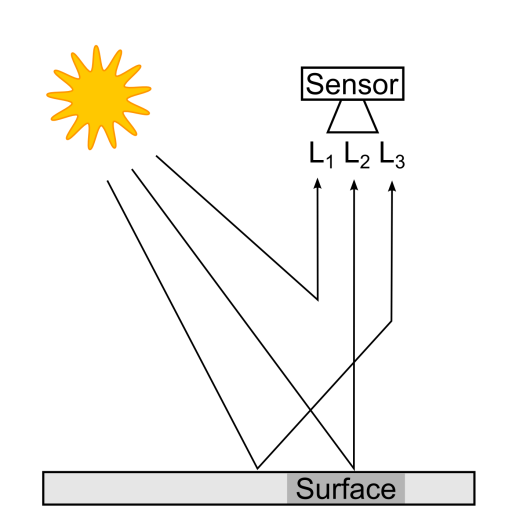
Schematic representation of radiation composition measured by the sensor. L1 = path radiance, L2 = reflected radiance, L3 = adjacency radiance.

Atmospheric corrections based on radiative transfer models allow for the calculation of absolute reflection without prior knowledge of surface reflective properties. This calculation is divided into two parts: estimation of atmospheric parameters and calculation of surface reflectance. The main atmospheric parameters relevant for atmospheric corrections are: the type and quantity of aerosols (AOT – Aerosol Optical Thickness) and the water vapor content. These are parameters that significantly affect the passage of radiation and can change over time. Atmospheric parameters can be measured using a sunphotometer within field support measurements or can be estimated directly from scanned data. The actual calculation of reflectance is then based on the look-up tables generated by the radiation transfer model. When modeling, the respective atmospheric transmittance is calculated for each wavelength, combination of atmospheric parameters and flight level. If we assume a flat terrain without adjacency effects and cloudless conditions, then the radiance at the sensor level (L) can be expressed as follows:

L = L1 + ρτE_g1/π

where L1 is the path radiation, ρ – surface reflectance, τ – transmittance of the atmosphere calculated as the sum of direct and diffusion transmittance, Eg – global irradiance at surface level, calculated as the sum of direct and diffusion irradiance for the zero reflection surface. Since all the members of the equation except ρ are known (measured or obtained from the model), it is possible to calculate the reflectance of the measured surface.

In order to exclude the influence of the current state of the atmosphere on the acquired data, in particular the effects of aerosols and atmospheric gases as described above, atmospheric corrections of scanned data are performed in the ATCOR-4 (ReSe Aplication Schlapfler/DLR) program using the MODRAN radiation transfer model of the atmosphere. During the corrections, both L1 path radiance and L3 adjacency radiance are corrected and the resulting reflectance is calculated from L2 (reflected radiance). The resulting atmospherically corrected data are expressed in reflectance values at surface level. In the data, reflectance values are multiplied by a constant of 100. I.e. the value of 1000 means reflectance of 10,00%.

To minimize the BRDF effect, the BREFCOR module is usually used. Its output is the correction of each pixel to the reflectance that it would have had if it had been scanned in the nadir. An example of two mosaicked flight lines without performing the correction in the BREFCOR module can be seen at MapServer.

More information about airborne remote sensing could be found in monograph Airborne remote sensing and in the article Flying Laboratory of Imaging Systems: Fusion of Airborne Hyperspectral and Laser Scanning for Ecosystem Research

Standard Outputs:

At surface reflectance in the spatial resolution of CASI sensor (spectral range 400-1000 nm)
At surface reflectance in the spatial resolution of the SASI sensor (spectral range 400-2400 nm)